readr
Basics
The Data Import cheat sheet reminds you how to read in flat files with http://readr.tidyverse.org/, work with the results as tibbles, and reshape messy data with tidyr. Use tidyr to reshape your tables into tidy data, the data format that works the most seamlessly with R and the tidyverse.
R’s tidyverse is built around tidy data stored in tibbles, an enhanced version of a data frame.
Readr read text files into R.
tidyr create tibbles with tibble and to layout tidy data.
Save Data
Save x, an R object, to path, a file path, as:
| func | name | delim | arguments |
|---|---|---|---|
| write_csv | Common delimited file | , | |
| write_delim | File with arbitrary delimiter | any | delim=“…” |
| write_excel_csv | CSV for excel | ||
| write_file | String to | ||
| write_lines | String vector to file | ||
| write_rds | Object to RDS file | compress=c(“none”,“gz”,“bz2”,“xz”) | |
| write_tsv | Tab delimited files | tab |
Read Tabular Data
These functions share the common arguments:
read_*(file, col_names=TRUE, col_types=NULL, locale=default_locale(), na=c(“”,“NA”), quoted_na=TRUE, comment=“”, trim_ws=TRUE, skip=0, n_max=inf, guess_max=min(1000, n_max), progress=interative())
Read tabular data tibbles
Comma Delimited files
write_file(x = "a,b,c\n1,2,3\n4,5,NA", path = "file.csv")
read_csv("file.csv")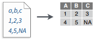
Semi-colon Delimited Files
write_file(x = "a;b;c\n1;2;3\n4;5;NA", path = "file2.csv")
read_csv2("file2.csv")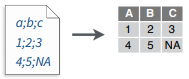
Files with Any Delimiter
write_file(x = "a|b|c\n1|2|3\n4|5|NA", path = "file.txt")
ead_delim("file.txt", delim = "|")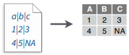
Fixed Width Files
write_file(x = "a b c\n1 2 3\n4 5 NA", path = "file.fwf")
read_fwf("file.fwf", col_positions = c(1, 3, 5))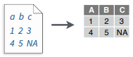
Tab Delimited Files
write_file(x = "a\tb\tc\n1\t2\t3\n4\t5\tNA", path = "file.tsv")
read_tsv("file.tsv") Also read_table()
Useful arguments
Example File
write_file("a,b,c\n1,2,3\n4,5,NA","file.csv")
f <- "file.csv" 
No header
read_csv(f, col_names = FALSE)
Provide header
read_csv(f, col_names = c("x", "y", "z"))
Skip lines
read_csv(f, skip = 1) 
Read in a subset
read_csv(f, n_max = 1) 
Missing Values
read_csv(f, na = c("1", "."))
Read Non-Tabular Data
Read a file into a single string
read_file(file, locale = default_locale())Read each line into its own string
read_lines(file, skip = 0, n_max = -1L, na = character(),
locale = default_locale(), progress = interactive())
Read each line into its own string
read_lines(file, skip = 0, n_max = -1L, na = character(),
locale = default_locale(), progress = interactive())
Read a file into a raw vector
read_file_raw(file)Read each line into a raw vector
read_lines_raw(file, skip = 0, n_max = -1L,
progress = interactive())
Read Apache style log files
read_log(file, col_names = FALSE, col_types = NULL, skip = 0, n_max = -1, progress = interactive())Data Types
readr functions guess the types of each column and convert types when appropriate (but will NOT convert strings to factors automatically). A message shows the type of each column in the result.
- Use problems() to diagnose problems.
x <- read_csv("file.csv"); problems(x) - Use a col_ function to guide parsing.
- col_guess() - the default
- col_character()
- col_double(), col_euro_double()
- col_datetime(format = “”) Also col_date(format = “”), col_time(format = “”)
- col_factor(levels, ordered = FALSE)
- col_integer()
- col_logical()
- col_number(), col_numeric()
- col_skip()
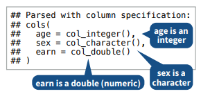
x <- read_csv("file.csv", col_types = cols(
 A = col_double(),
 B = col_logical(),
C = col_factor())) - Else, read in as character vectors then parse with a parse_ function.
- parse_guess()
- parse_character()
- parse_datetime() Also parse_date() and parse_time()
- parse_double()
- parse_factor()
- parse_integer()
- parse_logical()
- parse_number()
x$A <- parse_number(x$A)Tibbles
An enhanced data frame
The tibble package provides a new S3 class for storing tabular data, the tibble. Tibbles inherit the data frame class, but improve three behaviors:
- Subsetting - [ always returns a new tibble, [[ and $ always return a vector.
- No partial matching - You must use full column names when subsetting
- Display - When you print a tibble, R provides a concise view of the data that fits on one screen
- Control the default appearance with options:
options(tibble.print_max = n,
tibble.print_min = m, tibble.width = Inf)- View full data set with
View()orglimpse() - Revert to data frame with
as.data.frame()
CONSTRUCT A TIBBLE IN TWO WAYS
- tibble(…) - Construct by columns.
tibble(x = 1:3, y = c("a", "b", "c"))- tribble(…) - Construct by rows.
tribble( ~x, ~y,
 1, "a",
 2, "b",
 3, "c")
Other functions
Convert data frame to tibble.
as_tibble(x, …)Convert named vector to a tibble
enframe(x, name = "name", value = "value")Test whether x is a tibble.
is_tibble(x)
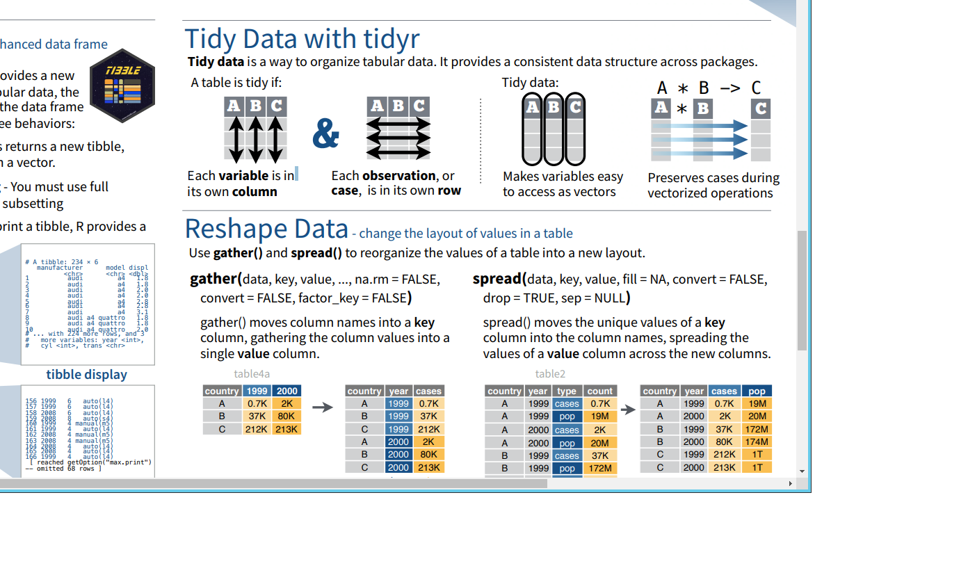
Tidy Data with tidyr
Tidy data is a way to organize tabular data. It provides a consistent data structure across packages.
- A table is tidy if:
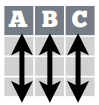
- Each variable is in its own column.
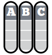
- Each observation, or case, is in its own row.

- Tidy Data:
- Makes variables easy to access as vectors.
- Preserves cases during vectorized operations.
Reshape Data
change the layout of values in a table
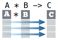
gather()moves column names into a key column, gathering the column values into a single value column.
gather(data, key, value, ..., na.rm = FALSE,
convert = FALSE, factor_key = FALSE)
gather(table4a, `1999`, `2000`,
key = "year", value = "cases") 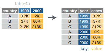
spread()moves the unique values of a key column into the column names, spreading the values of a value column across the new columns.
spread(data, key, value, fill = NA, convert = FALSE,
drop = TRUE, sep = NULL)
spread(table2, type, count)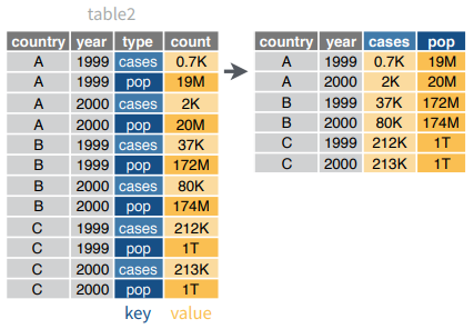
Handle Missing Values
drop_na(data, ...): Drop rows containing NA’s in … columns.
drop_na(x, x2)
fill(data, ..., .direction = c("down", "up")): Fill in NA’s in … columns with most recent non-NA values.
fill(x, x2)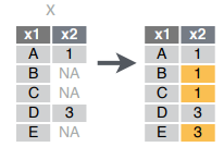
replace_na(data,replace = list(), ...): Replace NA’s by column.
replace_na(x, list(x2 = 2))
Expand Tables
quickly create tables with combinations of values
complete(data, ..., fill = list()): Adds to the data missing combinations of the values of the variables listed in …
complete(mtcars, cyl, gear, carb)expand(data, ...): Create new tibble with all possible combinations of the values of the variables listed in …
expand(mtcars, cyl, gear, carb)Split Cells
Use these functions to split or combine cells into individual, isolated values.
separate(data, col, into, sep = "[^[:alnum:]]+", remove = TRUE, convert = FALSE,
extra = "warn", fill = "warn", ...)
Separate each cell in a column to make several columns.
separate(table3, rate, into = c("cases", "pop"))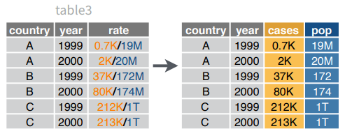
separate_rows(data, ..., sep = "[^[:alnum:].]+", convert = FALSE)Separate each cell in a column to make several rows. Also separate_rows_().
separate_rows(table3, rate)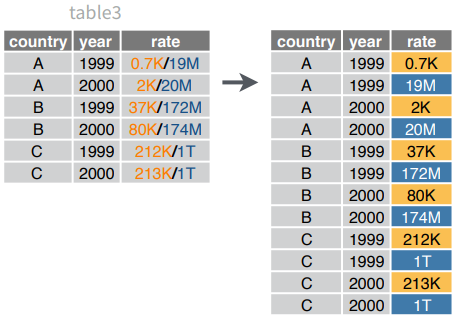
unite(data, col, ..., sep = "_", remove = TRUE)Collapse cells across several columns to make a single column.
unite(table5, century, year, col = "year", sep = "")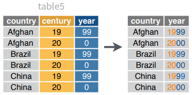
fread() for bigger datasets
- set working directory
- packages “data.table”
- handles large datasets fast
- easy to use
- improved .CSV importing features
- separator is automatically recognised
- strings are not automaticall convertied to factors | ‘stringsAsFactors=T’
- the header is displayed automaticall
- output: ‘data.frame’ (second class: ‘data.frame’) | ‘data.table=F’
library(data.table)
mydata = fread("./data/Bug-Frequency.csv")
mydatadf = fread("1 Singapore 5,612,300 710 7,905
2 Bangladesh 164,170,000 143,998 1,140
3 Taiwan 23,562,318 36,190 651
4 South Korea 51,446,201 99,538 517
5 Lebanon 6,082,000 10,452 582
6 Rwanda 11,809,295 26,338 448
7 Netherlands 17,200,000 41,526 414
8 Haiti 10,911,819 27,065 403
9 India 1,329,250,000 3,287,240 404
10 Israel 8,830,000 22,072 400",
col.names = c("Rank", "Country","Population", "Area(km2)","Density(Pop. per km2)"
))
dfdata.frame
- the mainly used object type
- straightforward sttucture
- one row for each observation
- one column for each variable
- R offers different data frame classes
- similar to R’s data visualization systems:
- ‘R-base’
- ‘lattice’
- ‘ggplot2’
- similar to R’s data visualization systems:
Three data frame alternatives
- ‘data.frame()’ function in ‘R-base’
- ‘data.table()’ function in the package ‘data.table’
- ‘data_frame()’ function in the package ‘dplyr’
each of them is suitabl for storing most data - Let’s see their specialities
data.frame
- no external package needed
- straightforward for simple tasks
- strings are stored as factors per default
- data recycling
- row names can be provided
mydf = data.frame(
    a = c("Paul", "Kim","Nora","Sue","Paul","Kim"),
    b = c("A", "B","C","B","B","C"),
    c = rnorm(2)
)
mydf
sapply(mydf, class)## a b c
## "factor" "factor" "numeric"data.table
- quick and easy to code
- start processing time
- great documentation
- second class ‘data.frame’
‘data.table’ struction is similar to SQL structure
- ‘nameDT [i, j, by]’
- ‘i’ stands for the subset from our ‘data.table’ we want to work with
- ‘j’ is the actual calculation that will be performed in the data subset ‘i’
- the whole calculation is grouped by ’by
- ‘nameDT [i, j, by]’
- strings are not automatically transfromed to factors
- no custom row names, just row IDs
if a dataset is too big to be processed, then only the first and last five rows are printed
library(data.table)
mytable = data.frame(
    a = c("Paul", "Kim","Nora","Sue","Paul","Kim"),
    b = c("A", "B","C","B","B","C"),
    c = rnorm(2)
)
mytable
data_frame
- requires equals column length
- only columns of length 1 will be recycled
- only the firs couple of rows are displayed in case of large datasets
- second class: ‘data.frame’
- stirngs are not automatically transformed to factors
- no custom row names, just row IDs
library(dplyr)
my_df = data.frame(
    a = c("Paul", "Kim","Nora","Sue","Paul","Kim"),
    b = c("A", "B","C","B","B","C"),
    c = rnorm(6)
)
my_df
Summary
class(mydf); class(mytable); class(my_df)## [1] "data.frame"## [1] "data.frame"## [1] "data.frame"- it is benefically to use advanced tools for extended data management
- ‘data.table’ and ‘data_frame’ have the standard ‘data.frame’ as second class
tibble
nycflights13
To explore the basic data manipulation verbs of dplyr, we’ll use nycflights13::flights. This data frame contains all 336,776 flights that departed from New York City in 2013. The data comes from the US Bureau of Transportation Statistics, and is documented in ?flights.
library(nycflights13)
flights
You might notice that this data frame prints a little differently from other data frames you might have used in the past: it only shows the first few rows and all the columns that fit on one screen. (To see the whole dataset, you can run
View(flights)which will open the dataset in the RStudio viewer). It prints differently because it’s a tibble. Tibbles are data frames, but slightly tweaked to work better in the tidyverse. For now, you don’t need to worry about the differences; we’ll come back to tibbles in more detail in wrangle.
You might also have noticed the row of three (or four) letter abbreviations under the column names. These describe the type of each variable:
intstands for integers.dblstands for doubles, or real numbers.chrstands for character vectors, or strings.dttmstands for date-times (a date + a time).lglstands for logical, vectors that contain onlyTRUEorFALSE.fctrstands for factors, which R uses to represent categorical variables with fixed possible values.datestands for dates.
‘scan()’ for small vectors and snippets
numbers = scan()
# characters = scan(what= "character")
Other types of data
Try one of the following packages to import other types of files.
- haven : SPSS, Stata, and SAS files
- readxl : excel files (.xls and .xlsx)
- DBI : databases
- jsonlite : json
- xml2 : XML
- httr : Web APIs
- rvest : HTML(Web Scraping)
packages ‘foreing’ to get help : ?foreign
?Hmisc
Alternatives
There are two main alternatives to readr: base R and data.table’s fread(). The most important differences are discussed below.
Base R
Compared to the corresponding base functions, readr functions:
Use a consistent naming scheme for the parameters (e.g.
col_namesandcol_typesnotheaderandcolClasses).Are much faster (up to 10x).
Leave strings as is by default, and automatically parse common date/time formats.
Have a helpful progress bar if loading is going to take a while.
All functions work exactly the same way regardless of the current locale. To override the US-centric defaults, use
locale().
data.table and fread()
data.table has a function similar to read_csv() called fread. Compared to fread, readr functions:
Are slower (currently ~1.2-2x slower. If you want absolutely the best performance, use
data.table::fread().Use a slightly more sophisticated parser, recognising both doubled (
"""") and backslash escapes ("\""), and can produce factors and date/times directly.Forces you to supply all parameters, where
fread()saves you work by automatically guessing the delimiter, whether or not the file has a header, and how many lines to skip.Are built on a different underlying infrastructure. Readr functions are designed to be quite general, which makes it easier to add support for new rectangular data formats.
fread()is designed to be as fast as possible.
These functions share the common arguments:
write_*(x, path, na=“NA”, append=FALSE, col_names=!append)