class: center, middle, inverse, title-slide # Base R --- exclude: true --- ## R as a Calculator .pull-left[ #### Basic calculation ```r 2+2 #> [1] 4 2^2 #> [1] 4 (1-2)*3 #> [1] -3 1-2*3 #> [1] -5 ``` #### Built-in Functions ```r sqrt(2) #> [1] 1.414214 sin(pi) #> [1] 1.224606e-16 exp(1) #> [1] 2.718282 log(10) #> [1] 2.302585 log(10, base=10) #> [1] 1 ``` ] .pull-right[ #### Variable Assignment ```r x = 2 # assignment x+3 #> [1] 5 pi # pi is a built-in constant #> [1] 3.141593 e^2 # Error #> Error in eval(expr, envir, enclos): 객체 'e'를 찾을 수 없습니다 e = exp(1) e^2 #> [1] 7.389056 (x <- 'apple') # print #> [1] "apple" ``` #### Getting Help ```r # 특정함수에 대한 도움말 보기 ?mean # 특정 용어"에 대한 도움말 검색 help.search('weighted mean') # 특정 패키지"에 대한 도움말 보기 help(package = 'deplyr') ``` ] --- ## (Almost) Everything is a Vector .pull-left[ #### Creating Vectors ```r # Join elements c(2, 4, 6) #> [1] 2 4 6 # An interger sequence 2:6 #> [1] 2 3 4 5 6 (2:6) * 0.3 #> [1] 0.6 0.9 1.2 1.5 1.8 # A complex sequence seq(2, 3, by=0.5) #> [1] 2.0 2.5 3.0 # Repeat a vector rep(1:2, times=3) #> [1] 1 2 1 2 1 2 # Repeat elements of a vector rep(1:2, each=3) #> [1] 1 1 1 2 2 2 rep(1:4, c(2,1,2,1)) #> [1] 1 1 2 3 3 4 rep(1:4, each=2, len=4) #> [1] 1 1 2 2 ``` ] .pull-right[ #### Vector function ```r x <- c(1, 3, 5, 2, 1, 5, 4, 6, 2, 5) # Return x sorted sort(x) #> [1] 1 1 2 2 3 4 5 5 5 6 # Return x reversed rev(x) #> [1] 5 2 6 4 5 1 2 5 3 1 # See counts of values table(x) #> x #> 1 2 3 4 5 6 #> 2 2 1 1 3 1 # See Unique values unique(x) #> [1] 1 3 5 2 4 6 ``` ] --- ## Maths Functions works for vectors ```r x <- c(1,2,3,4,5) y <- c(4,5,3,5,9) log(x) #> [1] 0.0000000 0.6931472 1.0986123 1.3862944 1.6094379 sum(x) #> [1] 15 exp(x) #> [1] 2.718282 7.389056 20.085537 54.598150 148.413159 round(exp(x), 2) #> [1] 2.72 7.39 20.09 54.60 148.41 mean(x) #> [1] 3 median(x) #> [1] 3 max(x) #> [1] 5 min(x) #> [1] 1 var(x) #> [1] 2.5 cor(x, y) #> [1] 0.6933752 sd(x) #> [1] 1.581139 rank(x) #> [1] 1 2 3 4 5 ``` --- ## Types of vectors The fundamental building block of data in R are vectors. R has two fundamental vector classes: - **atomic vectors** : *same* type elements ```r c(3, 4, 5) #> [1] 3 4 5 c("apple", "banana", "monkey") #> [1] "apple" "banana" "monkey" ``` - **Lists** : collections of *any* type of R object. ```r l <- list(3, list("apple","banana"), FALSE, 3.35) l #> [[1]] #> [1] 3 #> #> [[2]] #> [[2]][[1]] #> [1] "apple" #> #> [[2]][[2]] #> [1] "banana" #> #> #> [[3]] #> [1] FALSE #> #> [[4]] #> [1] 3.35 ``` --- ## R has six atomic vector types * logical : boolean values (TRUE or FALSE) * double : 2.44 * integer : 3L * character : "apple" * complex * raw ### How to convert types ```r a <- c(TRUE, FALSE, TRUE) print(a) #> [1] TRUE FALSE TRUE typeof(a) #> [1] "logical" a <- as.numeric(a) print(a) #> [1] 1 0 1 typeof(a) #> [1] "double" a <- as.logical(a) print(a) #> [1] TRUE FALSE TRUE typeof(a) #> [1] "logical" a <- as.character(a) print(a) #> [1] "TRUE" "FALSE" "TRUE" typeof(a) #> [1] "character" a <- as.factor(a) print(a) #> [1] TRUE FALSE TRUE #> Levels: FALSE TRUE typeof(a) #> [1] "integer" ``` --- ## Selecting Vector Elements - By Position ```r x <- c() x <- 1:6 x[4] #> [1] 4 x[-4] #> [1] 1 2 3 5 6 x[2:4] #> [1] 2 3 4 x[-(2:4)] #> [1] 1 5 6 x[c(1,3,5)] #> [1] 1 3 5 ``` - By Value ```r x[x==3] #> [1] 3 x[x<3] #> [1] 1 2 x[x %in% c(1,2,5)] #> [1] 1 2 5 ``` --- ## Condtions - a == b - a != b - a > b - a < b - a >= b - a <= b - is.na(a) - is.null(a) --- ## Comparisons Operator | Comparison | Vectorized? :-----------|:---------------------------|:----------------- `x < y` | less than | Yes `x > y` | greater than | Yes `x <= y` | less than or equal to | Yes `x >= y` | greater than or equal to | Yes `x != y` | not equal to | Yes `x == y` | equal to | Yes `x %in% y` | contains | Yes (for `x`) --- ## Logical (boolean) operations | Operator | Operation | Vectorized? |:-----------|:--------------|:------------- | <code>x &#124; y</code> | or | Yes | `x & y` | and | Yes | `!x` | not | Yes | <code>x &#124;&#124; y</code> | or | No | `x && y` | and | No |`xor(x,y)` | exclusive or | Yes --- --- ## Vectorized? ```r x = c(TRUE,FALSE,TRUE) y = c(FALSE,TRUE,TRUE) ``` .pull-left[ ```r x | y #> [1] TRUE TRUE TRUE x || y #> [1] TRUE ``` ] .pull-right[ ```r x & y #> [1] FALSE FALSE TRUE x && y #> [1] FALSE ``` ] --- ## handling data as a vector ```r typos.draft1 = c(2,2,3,4,5,3) typos.draft2 = typos.draft1 # make a copy typos.draft2[1] = 0 # assign the first value to 0 typos.draft2 #> [1] 0 2 3 4 5 3 typos.draft2[2] #> [1] 2 typos.draft2[4] #> [1] 4 typos.draft2 #> [1] 0 2 3 4 5 3 typos.draft2[-4] #> [1] 0 2 3 5 3 typos.draft2[c(1,2,5)] #> [1] 0 2 5 typos.draft2 == 3 #> [1] FALSE FALSE TRUE FALSE FALSE TRUE ``` --- ## Selecting some values with logical operators ```r typos = c(2,3,0,3,1,0,0,1) typos[typos==1] #> [1] 1 1 typos[typos>1] #> [1] 2 3 3 typos[typos<=1] #> [1] 0 1 0 0 1 typos[typos>0 & typos<=2] #> [1] 2 1 1 typos[typos<=0 | typos>2] #> [1] 3 0 3 0 0 ``` --- ## Matrix in R ```r # Generating Matrices matrix(1:8, ncol=4, nrow=2) #> [,1] [,2] [,3] [,4] #> [1,] 1 3 5 7 #> [2,] 2 4 6 8 matrix(c(1,2,3,11,12,13), nrow=2, ncol=3, byrow=T) #> [,1] [,2] [,3] #> [1,] 1 2 3 #> [2,] 11 12 13 matrix(c(1,2,3,11,12,13), nrow=2, ncol=3, byrow=TRUE, dimnames=list(c("row1","row2"),c("C.1","C.2","C.3"))) #> C.1 C.2 C.3 #> row1 1 2 3 #> row2 11 12 13 # Special Matrices diag(3) #> [,1] [,2] [,3] #> [1,] 1 0 0 #> [2,] 0 1 0 #> [3,] 0 0 1 diag(4:6) #> [,1] [,2] [,3] #> [1,] 4 0 0 #> [2,] 0 5 0 #> [3,] 0 0 6 A = matrix(0,3,3) A[upper.tri(A, diag=TRUE)] = 1:6 A #> [,1] [,2] [,3] #> [1,] 1 2 4 #> [2,] 0 3 5 #> [3,] 0 0 6 # Generating sub-matrices and sub-vectors A = matrix(1:9,3,3) A #> [,1] [,2] [,3] #> [1,] 1 4 7 #> [2,] 2 5 8 #> [3,] 3 6 9 A[,1] #> [1] 1 2 3 A[2,2] #> [1] 5 A[1,c(2,3)] #> [1] 4 7 A[1:2,2:3] #> [,1] [,2] #> [1,] 4 7 #> [2,] 5 8 ``` --- ## Operations ```r # Fundamental oprations of vectors c(1,3,5) + c(3,5,7) #> [1] 4 8 12 c(1,3,5) * c(3,5,7) #> [1] 3 15 35 c(1,3,5) / c(3,5,7) #> [1] 0.3333333 0.6000000 0.7142857 c(1,3,5) + 1 #> [1] 2 4 6 c(1,3,5) * 2 #> [1] 2 6 10 # Fundamental operations of matrices A = matrix(1:9,3,3) B = matrix(2:10,3,3) A;B #> [,1] [,2] [,3] #> [1,] 1 4 7 #> [2,] 2 5 8 #> [3,] 3 6 9 #> [,1] [,2] [,3] #> [1,] 2 5 8 #> [2,] 3 6 9 #> [3,] 4 7 10 A + B #> [,1] [,2] [,3] #> [1,] 3 9 15 #> [2,] 5 11 17 #> [3,] 7 13 19 A * B #> [,1] [,2] [,3] #> [1,] 2 20 56 #> [2,] 6 30 72 #> [3,] 12 42 90 A %*% B # matrix multiplication #> [,1] [,2] [,3] #> [1,] 42 78 114 #> [2,] 51 96 141 #> [3,] 60 114 168 t(A) #> [,1] [,2] [,3] #> [1,] 1 2 3 #> [2,] 4 5 6 #> [3,] 7 8 9 solve(A*B) #> [,1] [,2] [,3] #> [1,] 1.5 -2.5555556 1.1111111 #> [2,] -1.5 2.2777778 -0.8888889 #> [3,] 0.5 -0.7222222 0.2777778 solve(A*B) %*% (A*B) #> [,1] [,2] [,3] #> [1,] 1.000000e+00 -2.131628e-14 -4.263256e-14 #> [2,] 1.776357e-15 1.000000e+00 2.842171e-14 #> [3,] 0.000000e+00 -1.776357e-15 1.000000e+00 # Transformation of vectors and metrices A = matrix(1:4,2,2);A #> [,1] [,2] #> [1,] 1 3 #> [2,] 2 4 is.vector(A); is.matrix(A) #> [1] FALSE #> [1] TRUE as.vector(A) #> [1] 1 2 3 4 x = 1:3; y= 11:13 cbind(x,y) #> x y #> [1,] 1 11 #> [2,] 2 12 #> [3,] 3 13 rbind(x,y) #> [,1] [,2] [,3] #> x 1 2 3 #> y 11 12 13 ``` --- ## Data Frames ```r # Data frames and matrices A = matrix(1:4,2,2) dA = data.frame(A) dA #> X1 X2 #> 1 1 3 #> 2 2 4 is.matrix(dA) #> [1] FALSE is.data.frame(dA) #> [1] TRUE dA * dA #> X1 X2 #> 1 1 9 #> 2 4 16 dA %*% dA # does not work #> Error in dA %*% dA: 수치 또는 복소수형태의 행렬 혹은 벡터 인자가 요구됩니다 A %*% A #> [,1] [,2] #> [1,] 7 15 #> [2,] 10 22 # imported data set is a data frame dataset = read.csv("./data/data.csv", header=T, stringsAsFactors=F) head(dataset,5) #> AGE SEX #> 1 12 F #> 2 33 M #> 3 24 F #> 4 41 F #> 5 55 M is.data.frame(dataset) #> [1] TRUE is.matrix(dataset) #> [1] FALSE dataset[,1] #> [1] 12 33 24 41 55 dataset$AGE #> [1] 12 33 24 41 55 dataset$SEX #> [1] "F" "M" "F" "F" "M" ``` --- ## more about an object ```r data(iris) iris #> Sepal.Length Sepal.Width Petal.Length Petal.Width Species #> 1 5.1 3.5 1.4 0.2 setosa #> 2 4.9 3.0 1.4 0.2 setosa #> 3 4.7 3.2 1.3 0.2 setosa #> 4 4.6 3.1 1.5 0.2 setosa #> 5 5.0 3.6 1.4 0.2 setosa #> 6 5.4 3.9 1.7 0.4 setosa #> 7 4.6 3.4 1.4 0.3 setosa #> 8 5.0 3.4 1.5 0.2 setosa #> 9 4.4 2.9 1.4 0.2 setosa #> 10 4.9 3.1 1.5 0.1 setosa #> 11 5.4 3.7 1.5 0.2 setosa #> 12 4.8 3.4 1.6 0.2 setosa #> 13 4.8 3.0 1.4 0.1 setosa #> 14 4.3 3.0 1.1 0.1 setosa #> 15 5.8 4.0 1.2 0.2 setosa #> 16 5.7 4.4 1.5 0.4 setosa #> 17 5.4 3.9 1.3 0.4 setosa #> 18 5.1 3.5 1.4 0.3 setosa #> 19 5.7 3.8 1.7 0.3 setosa #> 20 5.1 3.8 1.5 0.3 setosa #> 21 5.4 3.4 1.7 0.2 setosa #> 22 5.1 3.7 1.5 0.4 setosa #> 23 4.6 3.6 1.0 0.2 setosa #> 24 5.1 3.3 1.7 0.5 setosa #> 25 4.8 3.4 1.9 0.2 setosa #> 26 5.0 3.0 1.6 0.2 setosa #> 27 5.0 3.4 1.6 0.4 setosa #> 28 5.2 3.5 1.5 0.2 setosa #> 29 5.2 3.4 1.4 0.2 setosa #> 30 4.7 3.2 1.6 0.2 setosa #> 31 4.8 3.1 1.6 0.2 setosa #> 32 5.4 3.4 1.5 0.4 setosa #> 33 5.2 4.1 1.5 0.1 setosa #> 34 5.5 4.2 1.4 0.2 setosa #> 35 4.9 3.1 1.5 0.2 setosa #> 36 5.0 3.2 1.2 0.2 setosa #> 37 5.5 3.5 1.3 0.2 setosa #> 38 4.9 3.6 1.4 0.1 setosa #> 39 4.4 3.0 1.3 0.2 setosa #> 40 5.1 3.4 1.5 0.2 setosa #> 41 5.0 3.5 1.3 0.3 setosa #> 42 4.5 2.3 1.3 0.3 setosa #> 43 4.4 3.2 1.3 0.2 setosa #> 44 5.0 3.5 1.6 0.6 setosa #> 45 5.1 3.8 1.9 0.4 setosa #> 46 4.8 3.0 1.4 0.3 setosa #> 47 5.1 3.8 1.6 0.2 setosa #> 48 4.6 3.2 1.4 0.2 setosa #> 49 5.3 3.7 1.5 0.2 setosa #> 50 5.0 3.3 1.4 0.2 setosa #> 51 7.0 3.2 4.7 1.4 versicolor #> 52 6.4 3.2 4.5 1.5 versicolor #> 53 6.9 3.1 4.9 1.5 versicolor #> 54 5.5 2.3 4.0 1.3 versicolor #> 55 6.5 2.8 4.6 1.5 versicolor #> 56 5.7 2.8 4.5 1.3 versicolor #> 57 6.3 3.3 4.7 1.6 versicolor #> 58 4.9 2.4 3.3 1.0 versicolor #> 59 6.6 2.9 4.6 1.3 versicolor #> 60 5.2 2.7 3.9 1.4 versicolor #> 61 5.0 2.0 3.5 1.0 versicolor #> 62 5.9 3.0 4.2 1.5 versicolor #> 63 6.0 2.2 4.0 1.0 versicolor #> 64 6.1 2.9 4.7 1.4 versicolor #> 65 5.6 2.9 3.6 1.3 versicolor #> 66 6.7 3.1 4.4 1.4 versicolor #> 67 5.6 3.0 4.5 1.5 versicolor #> 68 5.8 2.7 4.1 1.0 versicolor #> 69 6.2 2.2 4.5 1.5 versicolor #> 70 5.6 2.5 3.9 1.1 versicolor #> 71 5.9 3.2 4.8 1.8 versicolor #> 72 6.1 2.8 4.0 1.3 versicolor #> 73 6.3 2.5 4.9 1.5 versicolor #> 74 6.1 2.8 4.7 1.2 versicolor #> 75 6.4 2.9 4.3 1.3 versicolor #> 76 6.6 3.0 4.4 1.4 versicolor #> 77 6.8 2.8 4.8 1.4 versicolor #> 78 6.7 3.0 5.0 1.7 versicolor #> 79 6.0 2.9 4.5 1.5 versicolor #> 80 5.7 2.6 3.5 1.0 versicolor #> 81 5.5 2.4 3.8 1.1 versicolor #> 82 5.5 2.4 3.7 1.0 versicolor #> 83 5.8 2.7 3.9 1.2 versicolor #> 84 6.0 2.7 5.1 1.6 versicolor #> 85 5.4 3.0 4.5 1.5 versicolor #> 86 6.0 3.4 4.5 1.6 versicolor #> 87 6.7 3.1 4.7 1.5 versicolor #> 88 6.3 2.3 4.4 1.3 versicolor #> 89 5.6 3.0 4.1 1.3 versicolor #> 90 5.5 2.5 4.0 1.3 versicolor #> 91 5.5 2.6 4.4 1.2 versicolor #> 92 6.1 3.0 4.6 1.4 versicolor #> 93 5.8 2.6 4.0 1.2 versicolor #> 94 5.0 2.3 3.3 1.0 versicolor #> 95 5.6 2.7 4.2 1.3 versicolor #> 96 5.7 3.0 4.2 1.2 versicolor #> 97 5.7 2.9 4.2 1.3 versicolor #> 98 6.2 2.9 4.3 1.3 versicolor #> 99 5.1 2.5 3.0 1.1 versicolor #> 100 5.7 2.8 4.1 1.3 versicolor #> 101 6.3 3.3 6.0 2.5 virginica #> 102 5.8 2.7 5.1 1.9 virginica #> 103 7.1 3.0 5.9 2.1 virginica #> 104 6.3 2.9 5.6 1.8 virginica #> 105 6.5 3.0 5.8 2.2 virginica #> 106 7.6 3.0 6.6 2.1 virginica #> 107 4.9 2.5 4.5 1.7 virginica #> 108 7.3 2.9 6.3 1.8 virginica #> 109 6.7 2.5 5.8 1.8 virginica #> 110 7.2 3.6 6.1 2.5 virginica #> 111 6.5 3.2 5.1 2.0 virginica #> 112 6.4 2.7 5.3 1.9 virginica #> 113 6.8 3.0 5.5 2.1 virginica #> 114 5.7 2.5 5.0 2.0 virginica #> 115 5.8 2.8 5.1 2.4 virginica #> 116 6.4 3.2 5.3 2.3 virginica #> 117 6.5 3.0 5.5 1.8 virginica #> 118 7.7 3.8 6.7 2.2 virginica #> 119 7.7 2.6 6.9 2.3 virginica #> 120 6.0 2.2 5.0 1.5 virginica #> 121 6.9 3.2 5.7 2.3 virginica #> 122 5.6 2.8 4.9 2.0 virginica #> 123 7.7 2.8 6.7 2.0 virginica #> 124 6.3 2.7 4.9 1.8 virginica #> 125 6.7 3.3 5.7 2.1 virginica #> 126 7.2 3.2 6.0 1.8 virginica #> 127 6.2 2.8 4.8 1.8 virginica #> 128 6.1 3.0 4.9 1.8 virginica #> 129 6.4 2.8 5.6 2.1 virginica #> 130 7.2 3.0 5.8 1.6 virginica #> 131 7.4 2.8 6.1 1.9 virginica #> 132 7.9 3.8 6.4 2.0 virginica #> 133 6.4 2.8 5.6 2.2 virginica #> 134 6.3 2.8 5.1 1.5 virginica #> 135 6.1 2.6 5.6 1.4 virginica #> 136 7.7 3.0 6.1 2.3 virginica #> 137 6.3 3.4 5.6 2.4 virginica #> 138 6.4 3.1 5.5 1.8 virginica #> 139 6.0 3.0 4.8 1.8 virginica #> 140 6.9 3.1 5.4 2.1 virginica #> 141 6.7 3.1 5.6 2.4 virginica #> 142 6.9 3.1 5.1 2.3 virginica #> 143 5.8 2.7 5.1 1.9 virginica #> 144 6.8 3.2 5.9 2.3 virginica #> 145 6.7 3.3 5.7 2.5 virginica #> 146 6.7 3.0 5.2 2.3 virginica #> 147 6.3 2.5 5.0 1.9 virginica #> 148 6.5 3.0 5.2 2.0 virginica #> 149 6.2 3.4 5.4 2.3 virginica #> 150 5.9 3.0 5.1 1.8 virginica str(iris) #> 'data.frame': 150 obs. of 5 variables: #> $ Sepal.Length: num 5.1 4.9 4.7 4.6 5 5.4 4.6 5 4.4 4.9 ... #> $ Sepal.Width : num 3.5 3 3.2 3.1 3.6 3.9 3.4 3.4 2.9 3.1 ... #> $ Petal.Length: num 1.4 1.4 1.3 1.5 1.4 1.7 1.4 1.5 1.4 1.5 ... #> $ Petal.Width : num 0.2 0.2 0.2 0.2 0.2 0.4 0.3 0.2 0.2 0.1 ... #> $ Species : Factor w/ 3 levels "setosa","versicolor",..: 1 1 1 1 1 1 1 1 1 1 ... class(iris) #> [1] "data.frame" head(iris) #> Sepal.Length Sepal.Width Petal.Length Petal.Width Species #> 1 5.1 3.5 1.4 0.2 setosa #> 2 4.9 3.0 1.4 0.2 setosa #> 3 4.7 3.2 1.3 0.2 setosa #> 4 4.6 3.1 1.5 0.2 setosa #> 5 5.0 3.6 1.4 0.2 setosa #> 6 5.4 3.9 1.7 0.4 setosa ``` --- ## List ```r # Collections of vectors and matrices x1 = c(1,2,3) x2 = c(4,5,6,7) x3 = c(7,8,9,10,11) list(x1,x2,x3) #> [[1]] #> [1] 1 2 3 #> #> [[2]] #> [1] 4 5 6 7 #> #> [[3]] #> [1] 7 8 9 10 11 list(x1,x2,x3)[[1]] #> [1] 1 2 3 list(a=x1,b=x2,c=x3) #> $a #> [1] 1 2 3 #> #> $b #> [1] 4 5 6 7 #> #> $c #> [1] 7 8 9 10 11 list(a=x1,b=x2,c=x3)$a #> [1] 1 2 3 ``` ```r l <- list(x = 1:5, y = c('a', 'b')) l[[2]] #> [1] "a" "b" l[1] #> $x #> [1] 1 2 3 4 5 l$x #> [1] 1 2 3 4 5 l['y'] #> $y #> [1] "a" "b" ``` --- ## controls ```r # if statements x = -1 if(x>0){y="positive"} y #> [1] 11 12 13 if(x>0){y="positive"}else{y="nagative"} y #> [1] "nagative" ifelse(x>0, "positive","negative") #> [1] "negative" ``` --- ```r # for loops a=b=c() for (i in 1:5){ a[i] = i b[i] = a[i] + i^2 } a #> [1] 1 2 3 4 5 b #> [1] 2 6 12 20 30 M = matrix(NA,3,5) for (i in 1:3){ for(j in 1:5){ M[i,j] = i + j^3 } } M #> [,1] [,2] [,3] [,4] [,5] #> [1,] 2 9 28 65 126 #> [2,] 3 10 29 66 127 #> [3,] 4 11 30 67 128 ``` --- ```r # While and Repeat loops i=0; a=100 while(a[i+1]>0.01){ i=i+1 a[i+1] = a[i]/10 } i #> [1] 4 a #> [1] 1e+02 1e+01 1e+00 1e-01 1e-02 i=0;a=100 repeat{ i=i+1 a[i+1]=a[i]/10 if(a[i+1]<=0.01) break } i #> [1] 4 a #> [1] 1e+02 1e+01 1e+00 1e-01 1e-02 ``` --- ## Graph in R ```r #Histogram x = rnorm(10000) hist(x, prob=T, main="H", xlab="X", ylab="Y") ``` <!-- --> ```r hist(x, prob=T, breaks=10, xlim=c(-4,4), ylim=c(0,0.4)) ``` 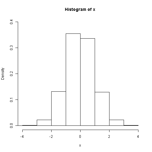<!-- --> ```r hist(x, prob=T, breaks=20, xlim=c(-4,4), ylim=c(0,0.4)) ``` <!-- --> ```r hist(x, prob=T, breaks=30, xlim=c(-4,4), ylim=c(0,0.4)) v=seq(-5,5,0.01) lines(v,dnorm(v)) lines(v,dnorm(v), col="blue") lines(v,dnorm(v), col="blue",lwd=4) ``` 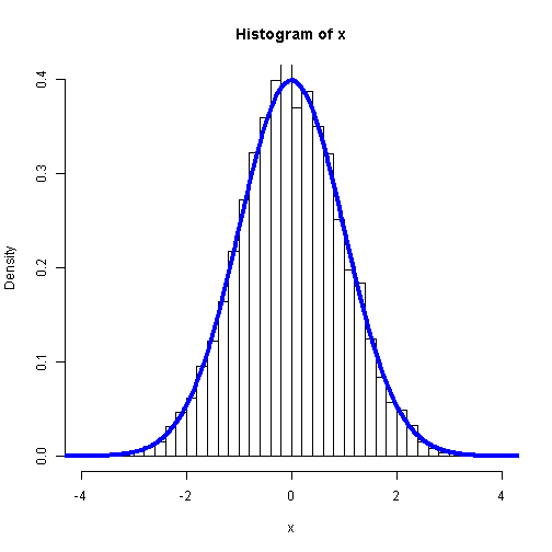<!-- --> --- ```r # Boxplots x = runif(10000, min=0, max=1) boxplot(x, main="Boxplot") ``` <!-- --> ```r head(OrchardSprays) #> decrease rowpos colpos treatment #> 1 57 1 1 D #> 2 95 2 1 E #> 3 8 3 1 B #> 4 69 4 1 H #> 5 92 5 1 G #> 6 90 6 1 F boxplot(decrease ~ treatment, data=OrchardSprays, col="bisque") ``` <!-- --> --- ```r # plot functions x = seq(-3,3,0.25) y = dnorm(x) plot(x,y) ``` 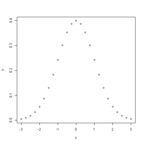<!-- --> ```r plot(x,y,type="l") ``` 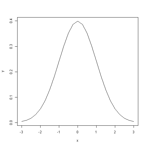<!-- --> ```r plot(x,y,type="h") points(x,y,pch=2) lines(x,y,lty=2) ``` <!-- --> --- ## Random number generations ```r x = rnorm(100000, mean=5, sd=5) hist(x, main="N(5,25)") abline(v=5, lty=2,lwd=3) ``` <!-- --> ```r y=rgamma(10000,shape=5,scale=5) hist(y,main="Gamma(5,5)") ``` <!-- --> --- ## functions in R ```r f1 = function(x,y,z) { x^2+log(y)+exp(z) } f1(2,3,4) #> [1] 59.69676 f2 = function(A,B){ temp = A %*% B det(temp) } A0 = matrix(1:4,2,2) B0 = matrix(5:8,2,2) f2(A0,B0) #> [1] 4 ``` --- ## Install Packages ```r # installing R packages # install.packages("ggplot2") # importing R packages library(ggplot2) ``` --- ## Working Directory ```r getwd() #> [1] "D:/Dropbox/DSHandbook/DSHub" #setwd('C://file/path') ``` --- ## Environment ```r rm(list = ls()) a <- "apple" b <- c(1,2,3) c <- 1 ls() #> [1] "a" "b" "c" rm(a) ls() #> [1] "b" "c" rm(list = ls()) ``` --- ## Reading a text file ```r # read csv read.csv("./data/data.csv", header=T, stringsAsFactors=F) #> AGE SEX #> 1 12 F #> 2 33 M #> 3 24 F #> 4 41 F #> 5 55 M # text file read.table("./data/data.txt") #> V1 #> 1 AGE|SEX #> 2 12|F #> 3 33|M #> 4 24|F #> 5 41|F #> 6 55|M read.table("./data/data.txt", header=T, sep="|", stringsAsFactors=F) #> AGE SEX #> 1 12 F #> 2 33 M #> 3 24 F #> 4 41 F #> 5 55 M ``` --- ## Read & Write data ```r ## create txt file # fileConn<-file("file.txt") # writeLines(c("Hello","World"), fileConn) # close(fileConn) df <- c("Hello","World") write.table(df, 'file2.txt') df2 <- read.table('file2.txt') print(df2) ``` ```r df <- c("apple","graph") write.csv(df, 'file3.csv') df3 <- read.csv('file3.csv') print(df3) ``` ```r df <- c("apple3","graph3") save(df, file = 'file4.Rdata') load('file4.Rdata') print(df) ``` --- ## Reference: - Ruey S. Tsay, An Introduction to Analysis of Financial Data with R - Taeyoung Park, Bayesian Inference & Computation